Next: Varianz und höhere Momente
Up: Momente von Zufallsvariablen
Previous: Momente von Zufallsvariablen
Contents
Erwartungswert
Bevor wir zur allgemeinen Definition des Erwartungswertes kommen,
wollen wir die intuitive Bedeutung dieses Begriffes anhand des
folgenden Beispiels erläutern.
- Beispiel
 (wiederholtes Würfeln)
- Betrachten den Wahrscheinlichkeitsraum
 mit der Grundmenge
und dem Wahrscheinlichkeitsmaß
mit der Grundmenge
und dem Wahrscheinlichkeitsmaß  , das durch
gegeben ist;
, das durch
gegeben ist;
 ;
;
 ;
;
 .
.
- Betrachten die Zufallsvariablen
 , die gegeben seien durch die
Projektion
, die gegeben seien durch die
Projektion
 für
für
 .
D.h.,
.
D.h.,  ist die (zufällige) Augenzahl, die beim
 -ten Würfeln erzielt wird.
- Es ist nicht schwierig zu zeigen,
daß
 unabhängige (und identisch verteilte)
Zufallsvariable sind.
unabhängige (und identisch verteilte)
Zufallsvariable sind.
- Betrachten die Zufallsvariable
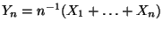 , d.h. die mittlere Augenzahl
bei
, d.h. die mittlere Augenzahl
bei  -maligem Würfeln.
- Man kann zeigen, daß es eine ,,nichtzufällige'' Zahl
 gibt,
so daß
gibt,
so daß
 |
(1) |
wobei
 |
(2) |
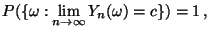
- Die Formeln (1) und (2) bedeuten:
Falls die Anzahl der durchgeführten Versuche immer größer
wird, dann
- werden die Werte
 der mittleren Augenzahl
  immer weniger
von der jeweiligen Ausprägung
immer weniger
von der jeweiligen Ausprägung  des Zufalls beeinflußt,
- strebt das ,,Zeitmittel'' bei Versuchen gegen das
,, Scharmittel'' c jedes (einzelnen) Versuches.
- Die Formeln (1) und (2) sind
ein Spezialfall des sogenannten Gesetzes
der großen Zahlen, das im weiteren Verlauf der Vorlesung noch
genauer diskutiert wird.
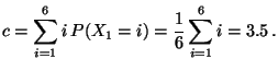
- Das Scharmittel
 in (2) wird Erwartungswert der
Zufallsvariablen
in (2) wird Erwartungswert der
Zufallsvariablen  genannt und mit
 bezeichnet.
Auf analoge Weise wird der Begriff des Erwartungswertes für
beliebige (diskrete bzw. absolutstetige) Zufallsvariable
eingeführt.
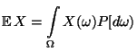
- Definition 4.1
- Betrachten einen beliebigen
Wahrscheinlichkeitsraum
 .
.
- Sei
 eine diskrete Zufallsvariable
mit
eine diskrete Zufallsvariable
mit
 für eine abzählbare Menge
 . Dann heißt das gewichtete Mittel
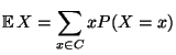 |
(3) |
der Erwartungswert von  ,
wobei vorausgesetzt wird, daß
,
wobei vorausgesetzt wird, daß
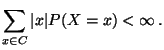 |
(4) |
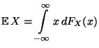
- Sei
eine absolutstetige Zufallsvariable
mit der Dichte
 . Dann heißt das Integral
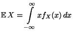 |
(5) |
der Erwartungswert von , wobei vorausgesetzt wird, daß
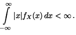 |
(6) |
- Beachte
-
- Beispiele
-
Wir zeigen nun anhand zweier Beipiele, wie
die Formeln (3) und (5) zur Bestimmung des
Erwartungswertes genutzt werden können.
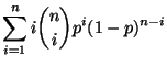
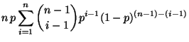
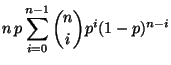
- Binomialverteilung
Sei binomialverteilt mit den Parametern
 und
und
![$ p\in[0,1]$](img310.png) . Dann ergibt sich aus (3), daß
. Dann ergibt sich aus (3), daß
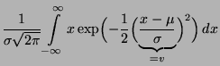
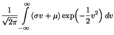
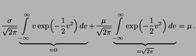
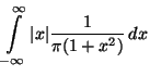
- Normalverteilung
Sei normalverteilt mit den
Parametern
 und
und  .
Dann ergibt sich aus (5), daß
.
Dann ergibt sich aus (5), daß
- Beachte
-
Next: Varianz und höhere Momente
Up: Momente von Zufallsvariablen
Previous: Momente von Zufallsvariablen
Contents
Roland Maier
2001-08-20
![$\displaystyle \frac{1}{\pi }\lim _{t\to\infty}
\left[\frac{1}{2}\log (1+x^{2})\right]_{0}^{t}
=\frac{1}{2\pi }\lim _{t\to\infty}\log (1+t^{2})=\infty\,.$](img744.png)