Definition and Basic Properties

Let $X=\{X_1,X_2,\ldots\}$ be a homogeneous Poisson process with intensity $\lambda$ and let $M=\{ M_0,M_1,\ldots\}$ be a sequence of independent and identically distributed random compact sets that are independent of the Poisson process X. The union $\Xi = \bigcup_{n\geq 1} (M_n + X_n)$of all shifted sets is called a Boolean model; see e.g. Hall (1988), Molchanov (1997), Stoyan et al. (1995), Weil (1988, 1995). The points X_i are sometimes called germs and the random set M₀ is said to be the `typical grain` of the Boolean model $\Xi$ (also called Poisson germ-grain model). 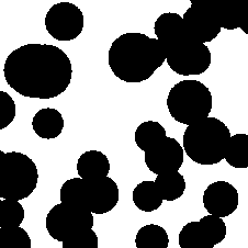A realization of a Boolean model where the sets M_n are discs with uniformly distributed radii R_n in a certain interval is given in Figure 6.

 

Figure 6:  Boolean model

An important characteristic of the Boolean model is the area fraction p, which is the mean fraction of area covered by $\Xi$in a region of unit area, i.e., $p = \Exp (\nu (\Xi \cap B))$ for $\nu(B) = 1$.Because of the stationarity of the Boolean model, this is also the probability that the origin o is covered by $\Xi$. By application of the Poisson assumption, p takes the form  

$$p = \Prob (o \in \Xi) = 1 - \exp(-\lambda \Exp (\nu(M_0))).$$ (10)

The Choquet theorem states that the distribution of $\Xi$ is uniquely determined by the so-called capacity functional $T_{\Xi}(K)$, which is the probability that $\Xi$ hits a fixed compact set $K \subset {\cal K}$, where ${\cal K}$ is the family of compact sets in $\RL^2$, i.e.,  

$$T_{\Xi}(K) = \Prob (\Xi \cap K \neq \emptyset), \qquad \qquad K \in {\cal K};$$ (11)

see Matheron (1975) for a proof of it.

Analogous to Section 2.1 the contact distribution function H^*_B(r) is defined for a convex set B containing the origin o as  

$$H^*_B(r) = 1 - \frac{\Prob (\Xi \cap rB = \emptyset)}{1-p} \qquad \mbox{ for } r \geq 0.$$ (12)

It holds that  

$$H^*_B(r) = 1 - \exp(-\lambda (\Exp (\nu (\check{M}_0 \oplus rB)) - \Exp (\nu (M_0)))) \qquad \mbox{ for } r \geq 0,$$ (13)

where $\check{M}_0 \oplus rB = \{ -x+y\, : \, x \in M_0, y \in rB\}$.In the special case where B is the unit disc, $H^*_B(r) \equiv H^*(r)$ is called the spherical contact distribution function.

Further quantities of interest are $p_0 = \Prob (X^* \mbox{ is covered by } \Xi^{\prime})$ and $p_G = \Prob (X^* + M^* \mbox{ intersects } \Xi^{\prime})$,where M^* is a `typical grain', X^* its corresponding germ and $\Xi^{\prime} = \bigcup \{ M_i + X_i \, : \, X_i \neq X^*\}$.These probabilities are given by p₀ = p and $p_G = 1 - \Exp (\exp(-\lambda \Exp(\nu(\check{M}_0 \oplus M_0))))$.If the grains are discs of fixed radius r, then $p_G = 1 - \exp(-\lambda \nu(b(o,2r)))$ and hence, using (4.10), p_G = 1-(1-p)⁴.

The number N of sets in the Boolean model that intersect a fixed convex subset S₀ of $\RL^2$is Poisson-distributed with mean  

$$\Exp (N) = \lambda \left\{ \nu (S_0) + \oA + \frac{1}{2\pi} \nu_1 (\partial S_0) \oU \right\},$$ (14)

where $\oA = \Exp (\nu (M_0))$, $\oU = \Exp(\nu_1 (\partial M_0))$,$\nu_1$ denotes the one-dimensional Lebesgue measure, and $\partial S_0$ the boundary of the set S₀. As a special case, the number N of sets in the Boolean model that cover the singleton $\{x\}$ is Poisson-distributed with mean $\Exp (N) = \lambda \oA$.It follows from (4.14) that the probability q(S₀) that S₀ has no intersection with $\Xi$ is given by  

$$q(S_0) = \exp \{ - \lambda [\oA + \nu (S_0) + \frac{1}{2\pi} \oU \nu_1(\partial S_0)]\}$$ (15)

in the case that S₀ is a fixed convex subset of $\RL^2$. If S₀ is a singleton, then  

$$q(S_0) = \exp \{ -\oA \lambda\}$$ (16)

and if S₀ is a line segment of length l, then  

$$q(S_0) = \exp \{ - \lambda ( \oA + \frac{l\oU}{\pi})\}.$$ (17)

For the Boolean model where the grains M_n are discs with independent identically distributed radii R_n with distribution function F, further Poisson processes can be assigned to (X,M): consider a fixed (deterministic) line $l \subset \RL^2$ and assume that $0 < \Exp R_n < \infty$. Then the sequence X_n^* of the projection on l of those points X_n such that the circle M_n + X_n hits the line l, forms a (one-dimensional) homogeneous Poisson process on l with intensity $2\lambda \Exp R_n$ (see Figure 7). Furthermore, the sequence X_n^* together with the sequence of intersections M_n^* of the discs M_n with the line l form a one-dimensional Boolean model $\Xi^*$.

 

Figure 7:  Intersection

The length of the intersections is distributed according to G with the density

$$\frac{dG(z)}{dz} = \frac{z}{\Exp (R_n)} \, \int_z^{\infty} \, (x^2 - z^2)^{-1/2} \; dF(x), \qquad z \gt 0.$$

Note that this construction of a linear Boolean model is also valid in a more general case, namely if the grains are convex sets. In the following we will restrict ourselves to discs.

The resulting pattern of clumps of intersection segments can be used to model a variety of phenomena. In mobile communications the two-dimensional Boolean model $\Xi$ can be interpreted as the users together with their power, where the germs are the locations of the callers and the grains are their random power. Hence the clumps of the associated one-dimensional Boolen model $\Xi^*$ can be interpreted as the regions of interference on the road and one is interested in the covered and uncovered parts of the road. The length of such an uncovered part is exponentially distributed with mean $1/\lambda_l$.The length of a typical clump has a distribution with Laplace-Stieltjes transform  

$$\gamma(s) = 1 + \frac{s}{\lambda_l} - \left( \lambda_l \int... ...ambda_l \int\limits_0^t \, (1-G(x))\,dx\right] dt \right)^{-1};$$ (18)

see e.g. Hall (1988). The distribution can be obtained numerically using an inversion algorithm for Laplace-Stieltjes transforms, for example the so-called Euler-algorithm; see e.g. Rolski et al. (1998).

In Frey (1997) the following approximation is given. For the distribution of the clump length L it holds that  

$$\Prob (L \gt x) = \sum_{i=0}^n \, \lambda_l^{i} \, \int\limits_0^{\infty} \, a_i(k,x) \, dG(k) \, + \, o(\lambda_l^n),$$ (19)

where the quantities a_i(k,x) are recursively given by  

$$a_0(k,x) = \left\{ \begin{array} {ll} 1 & \mbox{if } k\gt x \\ 0 & \mbox{else}\end{array}\right.$$ (20)

$$a_1(k,x) = \int\limits_0^k \, (1-G(x-t))\;dt$$ (21)

and for $i \geq 2$ 

$$a_i(k,x) = \int\limits_0^k \int\limits_{k-t}^{x-t} a_{i-1}(s,x-t) \, dG(s) - a_{i-1}(k-t,x-t) (1-G(k-t)) \, dt.$$ (22)

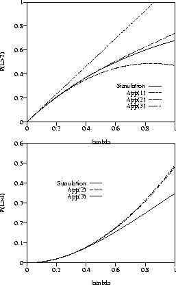
Figure 8 compares the above approximation with simulated values for x=2 (x=4 respectively) and

$$G(x) = \left\{ \begin{array} {ll} \sqrt{1- \frac{x^2}{4r^2}}... ... \leq x \leq 2r \\ 0 & x < 0 \\ 1 & x \gt 2r,\end{array}\right.$$

i.e., the radii of the discs in the two-dimensional Boolean model are fixed and equal to 1. By App(n) we mean the approximation by a polynomial of degree n given by (4.19).

 

Figure 8:   Approximations and simulation of the clump length distribution

From (4.19) one can deduce the probability that an interval of length t is completly covered by the one-dimensional Boolean model $\Xi^*$, i.e.,

where $\mu = \int_0^{\infty} \, x \, dG(x)$ and the quantities a_i(k,x) are given by (4.20) to (4.22).

Besides the distribution of the length of an uncovered part one is also interested in the distribution of the sum V of the uncovered parts in a given interval. Hall (1988) derived a formula for the distribution of vacancy V in the interval [0,t] provided that the segment length is fixed. However, this one-dimensional Boolean model cannot be deduced from a two-dimensional Boolean model. Frey (1997) showed for general distributed segment length and hence for a one-dimensional Boolean model which can be deduced from a two-dimensional Boolean model, that the distribution of vacancy V in [0,t] is given by

$$\Prob (V \leq x) = \sum_{i=1}^n \, \lambda^{i} a_{i}(-\infty,t,x) \, + \, o(\lambda^n),$$ (23)

provided that $\int_0^{\infty} \, s dG(s) < \infty$, where the quantities a_i(k,t,x) are recursively given by

$$a_1(k,t,x) = \int_k^0 \, \left( 1 - G(t-x-u)\right) \, du \, + \, \int_0^x \, \left( 1 - G(t-x) \right) \, du$$

and for $i \geq 2$

Similar problems where the grains are sticks were considered in Baszczyszyn et al. (1997), Rau (1997). They derived a Taylor-series expansion w.r.t. the intensity $\lambda$for the expectation of the typical clump length and calculated the first coefficients numerically.