


Next: Simulation Procedures
Up: Homogeneous Poisson Processes
Previous: Definition and Basic Properties
The estimation of the intensity  is the most fundamental
question in statistical analysis of homogeneous Poisson processes. There
are several approaches which are based on observing a sample of X
in a certain (bounded) observation window
is the most fundamental
question in statistical analysis of homogeneous Poisson processes. There
are several approaches which are based on observing a sample of X
in a certain (bounded) observation window  .
One of these approaches considers the number of points
lying in each of a set of n randomly or systematically located
sampling squares (or other subregions) of equal area, say a2.
Then, for observed counts
.
One of these approaches considers the number of points
lying in each of a set of n randomly or systematically located
sampling squares (or other subregions) of equal area, say a2.
Then, for observed counts  , a natural
estimator for is given by
, a natural
estimator for is given by
 .For n large and a2 small, another estimate of can be
obtained by computing the fraction
.For n large and a2 small, another estimate of can be
obtained by computing the fraction  of empty
squares and then by solving the equation
of empty
squares and then by solving the equation  .
We remark that in the literature
further estimators for are proposed which are based
on measuring the distances from sampling points
to certain neighboring points of the Poisson process, see e.g.
Diggle (1983, 1996), Ripley (1981).
.
We remark that in the literature
further estimators for are proposed which are based
on measuring the distances from sampling points
to certain neighboring points of the Poisson process, see e.g.
Diggle (1983, 1996), Ripley (1981).
A more fundamental statistical question is to test the hypothesis
that a given planar point pattern is a realization of a
homogeneous Poisson process. There exists a large number of
such tests which are based on different properties of the
Poisson process, see Stoyan et al. (1995).
Like the methods for estimating the intensity , one
can principially distinguish between tests based on measuring
distances between points and tests based on counting points.
The basis of tests where distance methods are used, is
(2.3), that is the fact that the spherical contact
distribution function H(r) of a homogeneous Poisson process
is equal to its nearest neighbor distance distribution function
D(r). In connection with this, one has to consider suitable
estimators for H(r) and D(r).
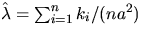
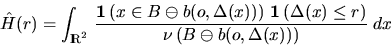
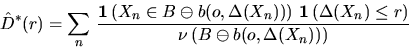
A simple unbiased estimator for H(r) is given by
|  |
(4) |
for  , where
  denotes the indicator function and b(x,r)
the circle with center x and radius r.
The symbol
denotes the indicator function and b(x,r)
the circle with center x and radius r.
The symbol  means Minkowski subtraction, i.e.,
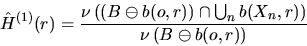
The estimator  and the set
  are
illustrated in Figure 2, where the estimator is the fraction of the shaded area to .
are
illustrated in Figure 2, where the estimator is the fraction of the shaded area to .
Figure 2:
The estimator and the set
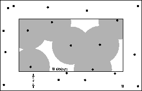 |
Note, however, that the estimator
given in (2.4) needs not to be monotone in r. Another
estimator for H(r) which does not have this disadvantage
goes back to an idea of
Hanisch (1984):
|  |
(5) |
for , where
 is the distance from x to its nearest neighbour
in
is the distance from x to its nearest neighbour
in  .
.
An asymptotically unbiased estimator for
D(r) which is
analogous to that in (2.4), is given by
| 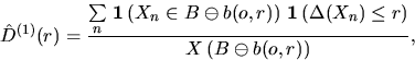 |
(6) |
which is the fraction of the number of points in whose nearest neighbor has distance less or equal to r, to the number
of points in .Again, this estimator needs not to be monotone in r. The following
estimator for D(r)
proposed by Hanisch (1984):
does not have this drawback:
| 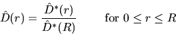 |
(7) |
where
and
 .
.
Now, the idea for testing the Poisson hypothesis on the basis of
(2.3) is to check
whether the empirical counterparts  and
and  of H(r) and D(r) respectively, computed from the observed point pattern,
are significantly different from each other; see also van Lieshout
and Baddeley (1996), Bedford and van den Berg (1997).
In Figure 3 this
method is illustrated using the data from Figure 1.
of H(r) and D(r) respectively, computed from the observed point pattern,
are significantly different from each other; see also van Lieshout
and Baddeley (1996), Bedford and van den Berg (1997).
In Figure 3 this
method is illustrated using the data from Figure 1.
Note that as usual in spatial
statistics, edge effects are an important component in the estimation
of H(r) and D(r). Such effects occur if the nearest neighbor of a point
lies outside of the observation window B.
In (2.5) and (2.7) an
edge-correction based on minus-sampling is considered, which
means that the estimators are based on subwindows  such that all neighbors with distance less than r
lie within the observation window B.
A new approach to edge corrected estimation
of D(r) has recently been presented in Floresroux and
Stein (1996).
Further related estimators for characteristics of planar point processes
can be found e.g. in Baddeley and Gill (1997),
Hansen et al. (1996,1998);
see also Jensen (1993).
such that all neighbors with distance less than r
lie within the observation window B.
A new approach to edge corrected estimation
of D(r) has recently been presented in Floresroux and
Stein (1996).
Further related estimators for characteristics of planar point processes
can be found e.g. in Baddeley and Gill (1997),
Hansen et al. (1996,1998);
see also Jensen (1993).
Another type of test for verifying the Poisson hypothesis is based
on the reduced second-order moment measure K of a
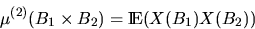
stationary point process X which is defined in the following way.
Note that this method can only be used in case of exhaustively mapped data,
i.e., when a complete set of the locations of all points in a pattern
is available. Assume that X has intensity and consider the second moment measure
|  |
(8) |
for  . Then, the reduced second-moment measure K
of X is uniquely determined by the equation
. Then, the reduced second-moment measure K
of X is uniquely determined by the equation
|  |
(9) |
If X is not only stationary but also isotropic, then K is
isotropic as well, and it suffices to consider the
reduced second-order moment function K(r) =
K(b(o,r)). Note that  can be interpreted as the
expected number of points in a circle with radius r and center at
the typical point of the point process. In the case that X is a homogeneous
Poisson process, (2.8) and (2.9) imply that
can be interpreted as the
expected number of points in a circle with radius r and center at
the typical point of the point process. In the case that X is a homogeneous
Poisson process, (2.8) and (2.9) imply that
 for all
  .
.
Assume now that a sample of X is observed in the window B,
 . Then, at first sight, a natural estimator
of
. Then, at first sight, a natural estimator
of  is
is

However, this estimator has an edge-bias since points which are close
to the boundary of B may have near neighbors outside B which
are not taken into account. The usual way one solves this problem
is to consider an edge-corrected estimator of the form
where k(x,y) is some weighting factor; see Ohser (1983),
Ripley (1988), Stein (1991, 1993),
Stoyan et al. (1995).
For example, a variant of  considered in
Ripley (1988) assumes that k-1(x,y) is the
proportion of the circumference of the circle with center x and
radius |x-y| which is contained in B.
considered in
Ripley (1988) assumes that k-1(x,y) is the
proportion of the circumference of the circle with center x and
radius |x-y| which is contained in B.
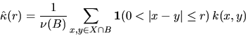
Now, an estimator for K(r) can be defined by
 where
where  is an estimator for .
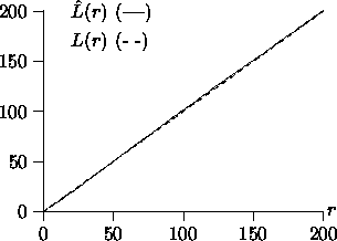
Note that for practical purposes, it is often more convenient
to consider the following L-function rather than K(r), where
 since L(r)=r in the Poisson case
which is a simple linear function, see Figure 4.
A natural test statistic for verifying
the Poisson process hypothesis is then
since L(r)=r in the Poisson case
which is a simple linear function, see Figure 4.
A natural test statistic for verifying
the Poisson process hypothesis is then
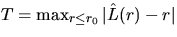 where
where  and r0 is an
upper bound for the interpoint distance r. If the value of T
is too large, then the Poisson hypothesis is doubted.
and r0 is an
upper bound for the interpoint distance r. If the value of T
is too large, then the Poisson hypothesis is doubted.
Figure 4:
Estimator  and L(r)=r
 |
If the data are observed in a rectangle, then a bivariate Cram'er-von Mises
type of test can be applied for testing the Poisson hypothesis. Suppose
that the points Xi have been observed in the window ![$[0,a] \times [0,b]$](img90.gif) ,a,b > 0, and are given in Cartesian coordinates
,a,b > 0, and are given in Cartesian coordinates
 and
and  , then the difference
 of the empirical bivariate distribution function and the
bivariate uniform distribution on can be used. The
difference has the computationally convenient representation
of the empirical bivariate distribution function and the
bivariate uniform distribution on can be used. The
difference has the computationally convenient representation
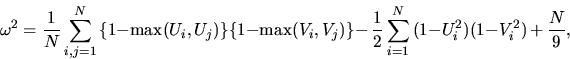
where N is the number of observed points in the rectangle
, Ui = Xi(1)/a and Vi = Xi(2)/b,
 . Its limiting distribution (
 ) under the Poisson hypothesis
was derived and tabulated by Durbin (1970).
Zimmermann (1993) extended this result by taking into account
that the realization of depends on which corner of the rectangle one chooses
as the origin. His quantity
) under the Poisson hypothesis
was derived and tabulated by Durbin (1970).
Zimmermann (1993) extended this result by taking into account
that the realization of depends on which corner of the rectangle one chooses
as the origin. His quantity
 which overcomes this difficulty has the form
see Zimmermann (1990, 1993)
for its limiting distribution under the Poisson hypothesis and selected percentiles of
its distribution.
We finally remark that besides the tests based on exhaustively mapped data,
there are tests which do not rely on a complete
set of the locations of all points. These so-called
quadrat count methods concern the case where the point pattern
is sampled by counting the numbers of points in several
(typically rectangular or quadratic) subregions of the observation
window and where the distributional properties of the counts under
the Poisson hypothesis are used; see Stoyan et al. (1995).
Next: Simulation Procedures
Up: Homogeneous Poisson Processes
Previous: Definition and Basic Properties
Andreas Frey
7/8/1998
