Transformation Algorithms for Discrete Distributions

• If pseudo-random numbers $x_1,x_2\ldots$ need to be generated
  • that can be regarded as realizations of discrete random variables $X_1,X_2\ldots$
  • taking the values $a_0,a_1\ldots\in\mathbb{R}$ with probabilities $p_j=P(X_i=a_j)\ge0$ for $j=0,1,\ldots$,
• then it is sometimes advisable to proceed as follows:
  • Let $U$ be a $(0,1]$-uniformly distributed random variable and let the random variable $X$ be given by

    $$X=\left\{\begin{array}{ll} a_0 &\mbox{if $U<p_0$,}\\ a_1 &\mbox{... ...ox{if $p_0+\ldots+p_{j-1}\le U<p_0+\ldots+p_j$,}\\ \vdots & \end{array}\right.$$ (13)

    
    

  • Then $P(X=a_j)=p_j$ for all $j=0,1,\ldots$.
• The pseudo-random numbers $x_1,\ldots,x_n$ where
  $$x_i=\left\{\begin{array}{ll} a_0 &\mbox{if $u_i<p_0$,}\\ a_0 &\... ...f $p_0+\ldots+p_{j-1}\le u_i<p_0+\ldots+p_j$,}\\ \vdots & \end{array}\right.$$
  • can thus be regarded as realizations of independent and ${\mathbf{p}}$-distributed random variables where
    ${\mathbf{p}}=(p_0,p_1,\ldots)^\top$,
  • if $u_1,\ldots,u_n$ are realizations of independent and uniformly distributed random variables on $(0,1]$.

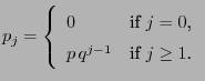
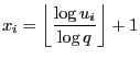
Example

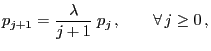
$\;$ (geometric distribution) 

• We consider the following values for $a_j$ and the corresponding probabilities $p_j$.
  • Let $a_j=j$ for $j=0,1,\ldots$, and for $0<p<1$ , $q=1-p$ let
    $$p_j=\left\{\begin{array}{ll} 0 & \mbox{if $j=0$,}\\ p\,q^{j-1} & \mbox{if $j\ge 1$.} \end{array}\right.$$

  • Then, for all $j\ge 1$,

    $$1-(p_1+\ldots+p_j)=p_{j+1}+p_{j+2}+\ldots=p\sum_{i=j}^\infty q^i=q^j$$ (14)

    
    
    and $p_j =q^{j-1}-q^j$.

  
  

• Furthermore, we consider the random variable

  $$X=\left\lfloor\frac{\log U}{\log q}\right\rfloor +1\,,$$ (15)

  
  
  where $U$ is a $(0,1]$-uniformly distributed random variable and $\left\lfloor z\right\rfloor$ denotes the integer part of $z$.

  
  

• Then $P(X=j)=p\,q^{j-1}$ for all $j=1,2,\ldots$, i.e. $X\sim$ Geo$(p)$,
  • as (14) and (15) imply
    

    $$X \stackrel{(\ref{for.peh.zwe})}{=} \min\Bigl\{j\ge 1:\,j>\;\frac{\log U}{\log q}\Bigr\}$$

    $$= \min\Bigl\{j\ge 1:\,j \log q <\log U\Bigr\}$$

    $$= \min\Bigl\{j\ge 1:\, q^j <U\Bigr\}$$

    $$= \sum\limits_{j=1}^\infty j\;{1\hspace{-1mm}{\rm I}}\bigl(q^j<U\le q^{j-1}\bigr)$$

    $$\stackrel{(\ref{for.peh.ein})}{=} \sum\limits_{j=1}^\infty j\;{1\hspace{-1mm}{\rm I}}\bigl(p_1+\ldots+p_{j-1}\le1-U<p_1+\ldots+p_j\bigr)\,,$$

    
    

  • where the random variable $1-U$ is also uniformly distributed on $(0,1]$.

  
  

• The pseudo-random numbers $x_1,\ldots,x_n$ where
  $$x_i=\left\lfloor\frac{\log u_i}{\log q}\right\rfloor +1$$
  • can thus be regarded as realizations of independent and geometrically distributed random variables $X_1,\ldots,X_n\sim$ Geo$(p)$
  • if $u_1,\ldots,u_n$ are realizations of independent random variables $U_1,\ldots,U_n$ that are uniformly distributed on the interval $(0,1]$.

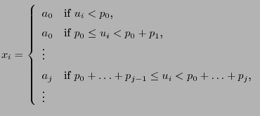
For some discrete distributions there are specific transformation algorithms allowing the generation of pseudo-random numbers having this distribution.

Examples

 

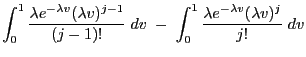
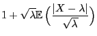
1. Poisson distribution $\;$ (with small expectation $\lambda$)
   • If $\lambda>0$ is a small number, then the following procedure is appropriate to generate Poisson-distributed pseudo-random numbers
     • by transformation of exponentially distributed pseudo-random numbers (as in Section 3.2.1)
     • or directly based on $(0,1]$-uniformly distributed pseudo-random numbers.
   • Let the random variables $X_1,X_2,\ldots$ be independent and Exp$(\lambda)$-distributed.
     • If we consider the random variable $Y=\max\{k\ge 0:\, X_1+\ldots+X_k\le 1\}$, formula (11) for the distribution function of the Erlang-distribution yields for all $j\ge 0$
       

       $$P(Y=j) = P(Y\ge j)-P(Y\ge j+1)$$

       $$= P(X_1+\ldots+X_j\le 1)-P(X_1+\ldots+X_{j+1}\le 1)$$

       $$= \int_0^1\displaystyle\frac{\lambda e^{-\lambda v}(\lambda v)^{j-1... ...dv\; -\;\int_0^1\displaystyle\frac{\lambda e^{-\lambda v}(\lambda v)^j}{j!}\;dv$$

       $$= \int_0^1\displaystyle\frac{d}{dv}\,\Bigl(\,\frac{ e^{-\lambda v}(\lambda v)^j}{j!}\,\Bigr)\,dv$$

       $$= \frac{ e^{-\lambda}\lambda^j}{j!}\;.$$

       
       

     • In other words we obtained $Y\sim$ Poi$(\lambda)$.
   • The pseudo-random numbers $y_1,\ldots,y_n$ where

     $$y_i = \max\{k\ge 0:\,x_1+\ldots+x_k\le i\}-y_{i-1}\,,\qquad\forall\, i=1,\ldots,n\,,$$ (16)

     
     
     and

     $$y_i = \max\{k\ge 0:\,u_1\cdot\ldots\cdot u_k\ge e^{-i\lambda}\}-y_{i-1}\,,\qquad\forall\, i=1,\ldots,n\,,$$ (17)

     
     
     where $y_0=0$ and $x_j=-\lambda^{-1}\log u_j$ for $j=1,2,\ldots$,
     • can thus be regarded as realizations of independent and Poi$(\lambda)$-distributed random variables,
     • if $x_1,x_2\ldots$ are realizations of Exp$(\lambda)$-distributed random variables $X_1,X_2\ldots$ and
     • if $u_1,\ldots,u_n$ are realizations of independent random variables $U_1,\ldots,U_n$ that are uniformly distributed on the interval $(0,1]$, respectively.
   • Remarks 
     • As the expectation of the Poi$(\lambda)$-distribution is given by $\lambda$, the mean number of uniformly distributed pseudo-random numbers necessary in order to generate a new Poi$(\lambda)$-distributed pseudo-random number is also $\lambda$.
     • For large $\lambda$ this effort can be reduced if one proceeds as follows.

   
   

2. Poisson distribution $\;$ (with large expectation $\lambda$)
   • If $\lambda>0$ is large, $a_j=j$ and $p_j=e^{-\lambda}\lambda^j/j!$ for $j=0,1,\ldots$,
     • then the procedure based directly on the transformation formula (13) is more appropriate to generate Poi$(\lambda)$-distributed pseudo-random numbers,
     • The validity of the inequalities

       $$U<p_0\,,\quad p_0\le U<p_0+p_1,\;\ldots,\; p_0+\ldots+p_{j-1}\le U<p_0+\ldots+p_j\,,\;\ldots$$ (18)

       
       
       needs to be checked in the order defined below.
     • Note that the recursion formula
       $$p_{j+1}=\frac{\lambda}{j+1}\;p_j\,,\qquad\forall\, j\ge 0\,,$$
       is applied to calculate the sums $P_j=\sum_{k=0}^j p_k$ for $j\ge 0$.
   • Let ${\left\lfloor \lambda\right\rfloor}>0$ be the integer part of $\lambda$. Then it is firstly checked if $U<P_{\left\lfloor \lambda\right\rfloor}$.
     • If this inequality holds it is checked if $U<P_{{\left\lfloor \lambda\right\rfloor}-1},U<P_{{\left\lfloor \lambda\right\rfloor}-2},\ldots$ where we define $X=\min\{k:\, U<P_k\}$.
     • If the inequality $U<P_{\left\lfloor \lambda\right\rfloor}$ does not hold then it is checked if $U<P_{{\left\lfloor \lambda\right\rfloor}+1},U<P_{{\left\lfloor \lambda\right\rfloor}+2},\ldots$ and we also define $X=\min\{k:\, U<P_k\}$.
   • For the expectation ${\mathbb{E}\,}V$ of the necessary number $V$ of checking steps we obtain the approximation
     

     $${\mathbb{E}\,}V \approx 1+{\mathbb{E}\,}\vert X-\lambda\vert$$

     $$= 1+\sqrt{\lambda}{\mathbb{E}\,}\Bigl(\frac{\vert X-\lambda\vert}{\sqrt{\lambda}}\Bigr)$$

     $$\approx 1+ 0.798\,\sqrt{\lambda}\,,$$

     
     
     • where the last approximation uses the fact that the random variable $(X-\lambda)/\sqrt{\lambda}$ is approximately N$(0,1)$-distributed for large $\lambda$ for the following reasons.
     • As the Poisson distribution is stabile under convolutions, i.e.,
       $${\rm Poi}(\lambda_1)*\ldots*{\rm Poi}(\lambda_n)={\rm Poi}\Bigl(\sum_{k=12}^n\lambda_i\Bigr)\,,$$
       the random variable $X\sim$ Poi$(\lambda)$ can be viewed as the sum $\sum_{i=1}^n X_i$ of $n$ independent and Poi $(\lambda/n)$-distributed random variables $X_i$. The last approximation then follows from the central limit theorem for sums of independent and identically distributed random variables; see Theorem WR-5.16.
   • We observe that
     • for increasing $\lambda$ the mean number of checking steps only grows with rate $\sqrt{\lambda}$ if this simulation procedure is applied,
     • whereas for the formerly discussed method generating Poi$(\lambda)$-distributed pseudo-random numbers the necessary number of standard pseudo-random numbers grows linearly in $\lambda$.

   
   

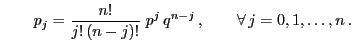
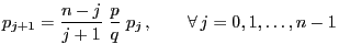
3. Binomial distribution 
   • For the generation of binomially distributed pseudo-random numbers one can proceed similarly to the Poisson case.
     • For arbitrary but fixed numbers $n\in\mathbb{N}$ and $p\in(0,1)$ where $q=1-p$ let
       $$a_j=j$$   and$$\qquad p_j=\frac{n!}{j!\,(n-j)!}\;p^j\,q^{n-j}\,,\qquad\forall\, j=0,1,\ldots,n\,.$$

     • For $j=0,1,\ldots,n$ the sums $P_j=\sum_{k=0}^j p_k$ are calculated via the recursion formula
       $$p_{j+1}=\frac{n-j}{j+1}\;\frac{p}{q}\;p_j\,,\qquad\forall\, j=0,1,\ldots,n-1$$

   • If $np>0$ is small, then
     • the validity of the inequalities (18) is checked in the natural order
     • starting at $U<p_0$ and defining $X=\min\{k:\, U<P_k\}$.
   • If $np$ is large,
     • then it is more efficient to check the validity of the inequalities (18) in the following order. It is firstly checked if $U<P_{\left\lfloor np\right\rfloor}$.
     • If this inequality holds it is checked if $U<P_{{\left\lfloor np\right\rfloor}-1},U<P_{{\left\lfloor np\right\rfloor}-2},\ldots$ where we also define $X=\min\{k:\, U<P_k\}$.
     • If the inequality $U<P_{\left\lfloor np\right\rfloor}$ does not hold it is checked if $U<P_{{\left\lfloor np\right\rfloor}+1},U<P_{{\left\lfloor np\right\rfloor}+2},\ldots$ where we again define $X=\min\{k:\, U<P_k\}$.