Next: Quotients of Uniformly Distributed
Up: Transformation of Uniformly Distributed
Previous: Transformation Algorithms for Discrete
Contents
Acceptance-Rejection Method
- In this section we discuss another method for the generation of
pseudo-random numbers

- First of all we consider the discrete case.
Theorem 3.5
- Let
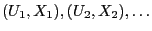 be a sequence of independent and
identically distributed random vectors whose components are
independent. Furthermore, let
be a sequence of independent and
identically distributed random vectors whose components are
independent. Furthermore, let  be a
be a ![$ (0,1]$](img165.png) -uniformly
distributed random variable and
-uniformly
distributed random variable and  be distributed according to
 .
.
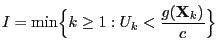
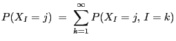
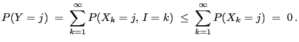
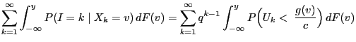
- Then
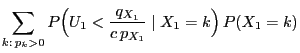
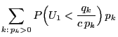
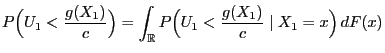
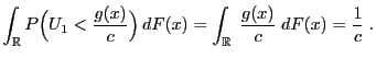
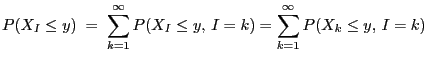
- Proof
-
- Remarks
-
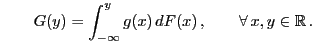
In the general (i.e. not necessarily discrete) case one can
proceed in a similar way. The following result will serve as
foundation for constructing acceptance-rejection algorithms.
- Proof
-
In the same way we obtain the following vectorial version of
Theorem 3.6.
- Examples
-
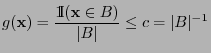
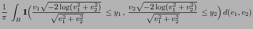
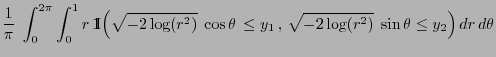
- Uniform distribution on bounded Borel sets
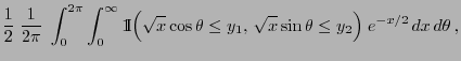
- Normal distribution
Next: Quotients of Uniformly Distributed
Up: Transformation of Uniformly Distributed
Previous: Transformation Algorithms for Discrete
Contents
Ursa Pantle
2006-07-20
![$\displaystyle G({\mathbf{y}})=\int_{(-\infty,{\mathbf{y}}]}\;\frac{{1\hspace{-1...
...}{\vert B\vert}\;dF({\mathbf{x}})\,,\qquad\forall\,{\mathbf{y}}\in\mathbb{R}^m
$](img1429.png)
 and
and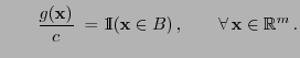


![$\displaystyle \qquad G({\mathbf{y}})=\int_{(-\infty,{\mathbf{y}}]} g({\mathbf{x...
...dF({\mathbf{x}})\,,\qquad \forall\, {\mathbf{x}},{\mathbf{y}}\in\mathbb{R}^m\,.$](img1420.png)