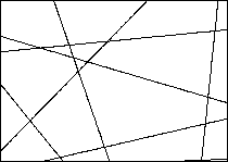
Now, let ![]() be an arbitrary stationary tessellation
which is not necessarily a Voronoi tessellation related to a point
process in
be an arbitrary stationary tessellation
which is not necessarily a Voronoi tessellation related to a point
process in ![]() .Then, C induces further stationary random sets which can be used
for analyzing communication networks: for example,
the edge-set E which is
a stationary segment process, and the stationary point processes
X(0), X(1), X(2) of nodes, edge-midpoints, and
cell-centroids
respectively. By
.Then, C induces further stationary random sets which can be used
for analyzing communication networks: for example,
the edge-set E which is
a stationary segment process, and the stationary point processes
X(0), X(1), X(2) of nodes, edge-midpoints, and
cell-centroids
respectively. By ![]() we denote the
intensity of X(i), i.e., the expected number of points
of X(i) per unit area, i=1,2,3. Note that
we denote the
intensity of X(i), i.e., the expected number of points
of X(i) per unit area, i=1,2,3. Note that ![]() . The intensity of E is traditionally denoted
by LA which is the expected total length of segments per unit area.
. The intensity of E is traditionally denoted
by LA which is the expected total length of segments per unit area.
Furthermore, let ![]() denote the expected number of
polygons touching the typical node of C,
denote the expected number of
polygons touching the typical node of C, ![]() the expected
total length of the edges emanating from that node,
the expected
total length of the edges emanating from that node, ![]() the expected length of the edge through the typical edge-midpoint,
the expected length of the edge through the typical edge-midpoint,
![]() the expected number of nodes on the boundary
of the cell containing the typical cell-centroid,
the expected number of nodes on the boundary
of the cell containing the typical cell-centroid, ![]() and
and ![]() the expected perimeter and area of that cell
respectively.
the expected perimeter and area of that cell
respectively.
All these expectations can be expressed by the three parameters
![]() and LA:
and LA:

Moreover, from the above formulae one obtains that
![]()
![]()
| |
(2) |
In the ordinary equilibrium state we further have
| |
(3) |
Relationships between characteristics of the typical cell of a stationary tessellation and its neighboring cells have been studied in Chiu (1994), Weiss (1995). Formulae for different types of contact distribution functions have been derived in Heinrich (1996), Last and Schassberger (1996, 1998) where also the chord length distribution of stationary (non-Poissonian) Voronoi tessellations is considered. In Heinrich and Muche (1997), representation formulae are given for the second factorial moment measure of the point process of nodes and the second moment of the number of edges of the typical cell associated with a stationary Voronoi tessellation in the ordinary equilibrium state.