


Next: Applications to Traffic Analysis
Up: Random Planar Tessellations
Previous: Stationary Tessellations
In this section, we assume that  is
a random Voronoi tessellation which is induced by a
homogeneous Poisson process
is
a random Voronoi tessellation which is induced by a
homogeneous Poisson process  with intensity
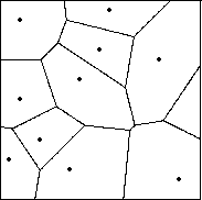
 (see Figure 12).
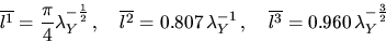
Then, the parameters
(see Figure 12).
Then, the parameters  and
LA are given by
and
LA are given by
|  |
(4) |
see e.g. Miles (1970). In particular,
 ,
,  and
and  .Further characteristics of the typical cell of a Poisson-Voronoi
tessellation can be obtained by using numerical integration and by
Monte Carlo simulation. For example,
in Møller (1994) and Stoyan et al. (1995),
see also Brakke (1985), Gilbert (1962),
Muche and Stoyan (1992), the following results are given.
Let
.Further characteristics of the typical cell of a Poisson-Voronoi
tessellation can be obtained by using numerical integration and by
Monte Carlo simulation. For example,
in Møller (1994) and Stoyan et al. (1995),
see also Brakke (1985), Gilbert (1962),
Muche and Stoyan (1992), the following results are given.
Let  and
and  denote the variance and the coefficient of variation
respectively of the positive random variable Z. Then
denote the variance and the coefficient of variation
respectively of the positive random variable Z. Then
Figure 12:
Tessellation
 |

where N02, L2, A2 denote the number of edges, the perimeter
and the area respectively of the typical Poisson-Voronoi cell.
Furthermore
|  |
(5) |
where  denotes the i-th moment of the length of the
typical chord generated by an intersection of the Poisson-Voronoi
tessellation with an arbitrary but fixed line. Note that alternatively one can
consider the moments of the length of the chord generated by a
`randomly chosen' test line
and the typical Poisson-Voronoi cell.
Miles and Maillardet (1982) determined the distribution of
the number of edges of the typical cell which can be useful in connection
with the problem of cochannel interference between cells (and optimal
channel assignment to the cells) of a cellular wireless communication system.
Note that this distribution does not depend on the intensity of the
underlying Poisson process Y. In Table 1, the probability
pn that the typical cell has n edges is given for some values
of n.
denotes the i-th moment of the length of the
typical chord generated by an intersection of the Poisson-Voronoi
tessellation with an arbitrary but fixed line. Note that alternatively one can
consider the moments of the length of the chord generated by a
`randomly chosen' test line
and the typical Poisson-Voronoi cell.
Miles and Maillardet (1982) determined the distribution of
the number of edges of the typical cell which can be useful in connection
with the problem of cochannel interference between cells (and optimal
channel assignment to the cells) of a cellular wireless communication system.
Note that this distribution does not depend on the intensity of the
underlying Poisson process Y. In Table 1, the probability
pn that the typical cell has n edges is given for some values
of n.
Table 1:
The distribution of the number of edges of
the typical Poisson-Voronoi cell
| n |
3 |
4 |
5 |
6 |
7 |
8 |
9 |
10 |
| pn |
0.011 |
0.107 |
0.259 |
0.295 |
0.199 |
0.090 |
0.030 |
0.007 |
In Hinde and Miles (1980) Monte Carlo simulation has been
used to obtain estimates for various further characteristics
of the typical cell of a Poisson-Voronoi tessellation.
For recent results on distributional properties related to the typical
Poisson-Voronoi cell, we refer to Mecke and Muche (1995),
Muche (1993, 1996, 1997),
and Muche and Stoyan (1992).
The density function of the half length  of the
typical Delaunay edge is given in Møller (1994):
of the
typical Delaunay edge is given in Møller (1994):
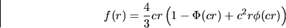
for  , where
  and
and  ,
, denote the density and distribution functions respectively
of the standard normal distribution. In particular
denote the density and distribution functions respectively
of the standard normal distribution. In particular
These results on characteristics of  can be used,
for instance to study
the cable length connecting two typical neighboring stations.
can be used,
for instance to study
the cable length connecting two typical neighboring stations.
Next: Applications to Traffic Analysis
Up: Random Planar Tessellations
Previous: Stationary Tessellations
Andreas Frey
7/8/1998