


Next: Optimization of Network Architecture
Up: Random Planar Tessellations
Previous: Poisson-Voronoi Tessellation
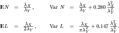
Assume that C0 is a random set which has the same distribution as the
typical cell of the Poisson-Voronoi tessellation  .Using (3.8) and (3.9) we can construct this cell in the
following way. It suffices to add a point at the origin to the underlying
Poisson process Y. Then, we can identify C0 with that cell of the
resulting Voronoi tessellation whose nucleus lies at the origin.
Now, besides Y, consider a further homogeneous Poisson process
.Using (3.8) and (3.9) we can construct this cell in the
following way. It suffices to add a point at the origin to the underlying
Poisson process Y. Then, we can identify C0 with that cell of the
resulting Voronoi tessellation whose nucleus lies at the origin.
Now, besides Y, consider a further homogeneous Poisson process
 with intensity
  which is
independent of Y and which can describe the locations of
subscribers. Many interesting characteristics, e.g. the
number N of subscribers being in the typical cell C0, have the form
which is
independent of Y and which can describe the locations of
subscribers. Many interesting characteristics, e.g. the
number N of subscribers being in the typical cell C0, have the form
 where
where  is a given nonnegative function. In order
to obtain N we simply put
is a given nonnegative function. In order
to obtain N we simply put  .Another example of such a characteristic is the sum L of the
distances between all subscribers in C0 and the nucleus of this cell
(being at the origin). In this case we take f(x) = |x|. Note that
.Another example of such a characteristic is the sum L of the
distances between all subscribers in C0 and the nucleus of this cell
(being at the origin). In this case we take f(x) = |x|. Note that
 .In the proof of this formula,
we use the fact that a point x belongs to C0 if and only
if there is no point of Y in the circle with radius |x|
and center at x; see Foss and Zuyev (1996). In particular,
.In the proof of this formula,
we use the fact that a point x belongs to C0 if and only
if there is no point of Y in the circle with radius |x|
and center at x; see Foss and Zuyev (1996). In particular,
Furthermore it is shown in Foss and Zuyev (1996)
that
and that similar inequalities hold for the tail function of L
as well; see also Baccelli et al. (1996). Analogous formulas
have been derived in Baccelli and Zuyev (1997) for
a spatial road traffic model, where
the random number of mobiles crossing the boundary of
the typical cell C0 in a fixed (small) period of time is considered.
Some details of this model will be discussed in Frey and
Schmidt (1997).
An extended point process model for communication networks with more than
two levels of hierarchy has been studied in Baccelli
et al. (1996); see also Baccelli and Zuyev (1998).
Assume that there are k+1 different levels of hierarchy, where
the subscribers are called 0-level stations, the stations
directly connected to 0-level stations are called 1-level stations,
and so on (see Figure 13).
Figure 13:
Communication network with three
levels of hierarchy
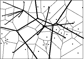 |
The locations of the stations of level i are represented
by a realization of a homogeneous Poisson process  with intensity
  . Assume that the Poisson processes
 are independent and
  . Furthermore, assume that
except for stations of level k, stations with the same level
have no direct connection between them. As in the model with two
hierarchy levels which we considered before, the stations of
level i (
. Furthermore, assume that
except for stations of level k, stations with the same level
have no direct connection between them. As in the model with two
hierarchy levels which we considered before, the stations of
level i ( ) are connected to their closest
station of level i+1. Thus, for each level
) are connected to their closest
station of level i+1. Thus, for each level  ,we consider the Poisson-Voronoi tessellation induced by X(i) and the
stations of level i-1 contained in the cell with nucleus Xn(i)
are directly connected to the latter.
,we consider the Poisson-Voronoi tessellation induced by X(i) and the
stations of level i-1 contained in the cell with nucleus Xn(i)
are directly connected to the latter.
This model has been used in Baccelli et al. (1996) to investigate
the demand for service in multi-level hierarchical communication systems.
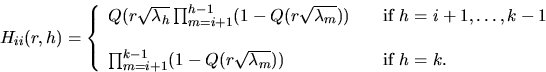
In connection with this the probability Hij(r,h) is considered
to have a communication of a height h between two fixed stations
of level i and j respectively which are located in distance r
from each other. Here the height h is defined as the minimal level
 such that two stations belong to the same
Voronoi cell induced by X(h). If there is no such h,
then h is set equal to the highest level, i.e,. h=k.
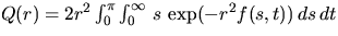
In order to determine the probabilities Hij(r,h), the tail
function Q(r) of the linear contact distribution function
of a normalized Poisson-Voronoi tessellation can be used. That is, let
Q(r) be the probability that two fixed points in the plane,
distant by r, belong to the same Voronoi cell induced by a
homogeneous Poisson process with intensity 1. Then
such that two stations belong to the same
Voronoi cell induced by X(h). If there is no such h,
then h is set equal to the highest level, i.e,. h=k.
In order to determine the probabilities Hij(r,h), the tail
function Q(r) of the linear contact distribution function
of a normalized Poisson-Voronoi tessellation can be used. That is, let
Q(r) be the probability that two fixed points in the plane,
distant by r, belong to the same Voronoi cell induced by a
homogeneous Poisson process with intensity 1. Then
 ,where

see e.g. Baccelli et al. (1996), Meijering (1953),
Muche and Stoyan (1992). On the other hand, Hij(r,h)
can be expressed by the tail function Q(r):
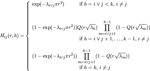
and analogously
The probabilities Hij(r,h) can be used to determine the
traffic matrix (nij(h),  where nij(h) denotes the expected number of
communications of height h per time unit between a fixed station
of level i to stations of level j. Namely,
where nij(h) denotes the expected number of
communications of height h per time unit between a fixed station
of level i to stations of level j. Namely,
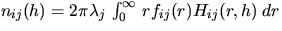 ,where fij(r) is the expected number of communications per time
unit which a station of level i asks for with a station of level j.
,where fij(r) is the expected number of communications per time
unit which a station of level i asks for with a station of level j.
Next: Optimization of Network Architecture
Up: Random Planar Tessellations
Previous: Poisson-Voronoi Tessellation
Andreas Frey
7/8/1998