Nächste Seite: Maximum-Likelihood-Gleichung und numerische Lösungsansätze
Aufwärts: Maximum-Likelihood-Schätzer für
Vorherige Seite: Loglikelihood-Funktion und ihre partiellen
Inhalt
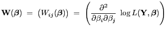
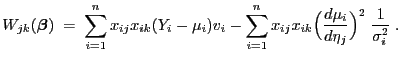
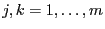
Hesse-Matrix
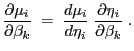
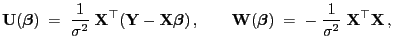
Neben dem (Score-) Vektor
 der ersten partiellen
Ableitungen der Loglikelihood-Funktion
der ersten partiellen
Ableitungen der Loglikelihood-Funktion
 wird auch ihre Hesse-Matrix, d.h., die
  -Matrix
der zweiten partiellen Ableitungen benötigt.
Theorem 4.2
- Für jedes GLM gilt
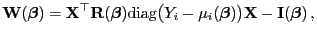 |
(34) |
wobei
 die in
 gegebene
Fisher-Informationsmatrix und
gegebene
Fisher-Informationsmatrix und
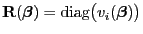 eine
eine
 -Diagonalmatrix ist mit
und
- Für GLM mit natürlicher Linkfunktion gilt insbesondere
 |
(35) |
- Beweis
-
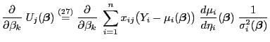
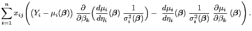
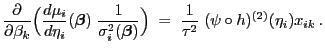
- Aus Formel (27) in Theorem 4.1 ergibt
sich, dass für beliebige
- Dabei ergibt sich mit der Schreibweise
 aus Lemma 4.2, dass
und somit
aus Lemma 4.2, dass
und somit
- Außerdem gilt
- Insgesamt ergibt sich also, dass
- Hieraus und aus der Darstellungsformel (29) für die
Fisher-Informationsmatrix
ergibt sich
(34).
- Weil für GLM mit natürlicher Linkfunktion die Superposition
 die Identitätsabbildung ist, gilt in diesem Fall
 . Somit ergibt sich (35)
aus (34).
. Somit ergibt sich (35)
aus (34).

- Beachte
 Für die Beispiele von GLM, die in
Abschnitt 4.2 betrachtet worden sind, ergeben sich
aus den Theoremen 4.1 und 4.2 bzw. aus
Korollar 4.1 die folgenden Formeln für
und
Für die Beispiele von GLM, die in
Abschnitt 4.2 betrachtet worden sind, ergeben sich
aus den Theoremen 4.1 und 4.2 bzw. aus
Korollar 4.1 die folgenden Formeln für
und
 .
.
- 1.
- Für das lineare Modell
 mit normalverteilten
Stichprobenvariablen (und mit der Linkfunktion
mit normalverteilten
Stichprobenvariablen (und mit der Linkfunktion  ) ist
) ist
 die Einheitsmatrix. Somit gilt
 |
(36) |
vgl. auch Abschnitt 2.2.
- 2.
- Für das logistische Regressionsmodell (mit der
natürlichen Linkfunktion) gilt
 |
(37) |
wobei
 und die
Wahrscheinlichkeiten
und die
Wahrscheinlichkeiten  so wie in (20) durch
 ausgedrückt werden können.
- 3.
- Für Poisson-verteilte Stichprobenvariablen mit
natürlicher Linkfunktion gilt
 |
(38) |
wobei
 und
und
 .
.
Nächste Seite: Maximum-Likelihood-Gleichung und numerische Lösungsansätze
Aufwärts: Maximum-Likelihood-Schätzer für
Vorherige Seite: Loglikelihood-Funktion und ihre partiellen
Inhalt
Hendrik Schmidt
2006-02-27