Metropolis-Hastings Algorithm

• We will now show that the Gibbs sampler discussed in Section 3.3.2 is a special case of a class of MCMC algorithms that are of the so-called Metropolis-Hastings type. This class generalizes two aspects of the Gibbs sampler.
  1. The transition matrix ${\mathbf{P}}=(p_{{\mathbf{x}}{\mathbf{x}}^\prime})$ can be of a more general form than the one defined by

     $$p_{{\mathbf{x}}{\mathbf{x}}^\prime}=\sum\limits_{v\in V} q_v \pi_... ...f{x}}^\prime(-v)\bigr)\,,\qquad\forall\, {\mathbf{x}},{\mathbf{x}}^\prime\in E.$$ (46)

     
     

  2. Besides this, a procedure for acceptance or rejection of the updates ${\mathbf{x}}\longrightarrow{\mathbf{x}}^\prime$ is integrated into the algorithm. It is based on a similar idea as the acceptance-rejection sampling discussed in Section 3.2.3; see in particular Theorem 3.5.

  
  

• Let $V$ be a finite nonempty index set and let ${\mathbf{X}}=(X(v),\,v\in V)$ be a discrete random vector,
  • taking values in the finite state space $E\subset\mathbb{R}^{\vert V\vert}$ with probability $1$.
  • As usual we assume $\pi_{\mathbf{x}}>0$ for all ${\mathbf{x}}\in E$ where ${\boldsymbol{\pi}}=(\pi_{\mathbf{x}},\,{\mathbf{x}}\in E)$ is the probability function of the random vector ${\mathbf{X}}$.
• We construct a Markov chain ${\mathbf{X}}_0,{\mathbf{X}}_1,\ldots$ with ergodic limit distribution ${\boldsymbol{\pi}}$ whose transition matrix ${\mathbf{P}}=\bigl(p_{{\mathbf{x}}{\mathbf{x}}^\prime}\bigr)$ is given by

  $$p_{{\mathbf{x}}{\mathbf{x}}^\prime}=q_{{\mathbf{x}}{\mathbf{x}}^\... ...{\mathbf{x}}^\prime}\,, \qquad\forall\, {\mathbf{x}},{\mathbf{x}}^\prime\in E\; \mbox{with ${\mathbf{x}}\not={\mathbf{x}}^\prime$,}$$ (47)

  
  
  • where ${\mathbf{Q}}=\bigl(q_{{\mathbf{x}}{\mathbf{x}}^\prime}\bigr)$ is an arbitrary stochastic matrix that is irreducible and aperiodic, i.e. in particular $q_{{\mathbf{x}}{\mathbf{x}}^\prime}=0$ if and only if $q_{{\mathbf{x}}^\prime{\mathbf{x}}}=0$.
  • Moreover, the matrix ${\mathbf{A}}=\bigl(a_{{\mathbf{x}}{\mathbf{x}}^\prime}\bigr)$ is defined as

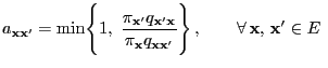
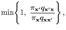
    $$a_{{\mathbf{x}}{\mathbf{x}}^\prime}=\frac{s_{{\mathbf{x}}{\mathbf{x}}^\prime}}{1+t_{{\mathbf{x}}{\mathbf{x}}^\prime}}\;,$$ (48)

    
    
    where

    $$t_{{\mathbf{x}}{\mathbf{x}}^\prime}=\left\{\begin{array}{ll}\disp... ...3\jot] 0 &\mbox{if $q_{{\mathbf{x}}{\mathbf{x}}^\prime}=0$,} \end{array}\right.$$ (49)

    
    

  • and ${\mathbf{S}}=\bigl(s_{{\mathbf{x}}{\mathbf{x}}^\prime}\bigr)$ is an arbitrary symmetric matrix such that

    $$0< s_{{\mathbf{x}}{\mathbf{x}}^\prime}\le 1+\min\,\bigl\{t_{{\mathbf{x}}{\mathbf{x}}^\prime}\,,t_{{\mathbf{x}}^\prime{\mathbf{x}}}\bigr\}\,.$$ (50)

    
    

Remarks

 

• The structure given by (47) of the transition matrix ${\mathbf{P}}=\bigl(p_{{\mathbf{x}}{\mathbf{x}}^\prime}\bigr)$ can be interpreted as follows.
  • At first a candidate ${\mathbf{x}}^\prime\in E$ for the update ${\mathbf{x}}\longrightarrow{\mathbf{x}}^\prime$ is selected according to ${\mathbf{Q}}=\bigl(q_{{\mathbf{x}}{\mathbf{x}}^\prime}\bigr)$.
  • If ${\mathbf{x}}^\prime\not={\mathbf{x}}$, then ${\mathbf{x}}^\prime$ is accepted with probability $a_{{\mathbf{x}}{\mathbf{x}}^\prime}$,
  • i.e., with probability $1-a_{{\mathbf{x}}{\mathbf{x}}^\prime}$ the update ${\mathbf{x}}\longrightarrow{\mathbf{x}}^\prime$ is rejected (and the current state is thus not changed).
• In order to apply the Metropolis-Hastings algorithm defined by (47)-(50), for a given ,,potential'' transition matrix ${\mathbf{Q}}=\bigl(q_{{\mathbf{x}}{\mathbf{x}}^\prime}\bigr)$ only the quotients $\pi_{\mathbf{x}}/\pi_{{\mathbf{x}}^\prime}$ need to be known for all pairs ${\mathbf{x}},\,{\mathbf{x}}^\prime\in E$ of states such that $q_{{\mathbf{x}}{\mathbf{x}}^\prime}>0$.
• The special case of the Gibbs sampler (see Section  3.3.2) is obtained
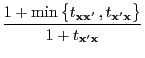
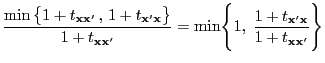
  • if the ,,potential'' transition probabilities $q_{{\mathbf{x}}{\mathbf{x}}^\prime}$ are defined by (46).
  • Then for arbitrary ${\mathbf{x}},\,{\mathbf{x}}^\prime\in E$ such that $\char93 \{v\in V:\,x(v)\not=x^\prime(v)\}\le 1$
    $$\pi_{\mathbf{x}}q_{{\mathbf{x}}{\mathbf{x}}^\prime}= \pi_{{\mathbf{x}}^\prime}q_{{\mathbf{x}}^\prime{\mathbf{x}}}$$   and thus$$\qquad t_{{\mathbf{x}}{\mathbf{x}}^\prime}=1\,.$$

  • By defining $s_{{\mathbf{x}}{\mathbf{x}}^\prime}= 1+\min\,\bigl\{t_{{\mathbf{x}}{\mathbf{x}}^\prime}\,,t_{{\mathbf{x}}^\prime{\mathbf{x}}}\bigr\}$ we obtain $a_{{\mathbf{x}}{\mathbf{x}}^\prime}=1$ for arbitrary ${\mathbf{x}},\,{\mathbf{x}}^\prime\in E$ such that $\char93 \{v\in V:\,x(v)\not=x^\prime(v)\}\le 1$.

Theorem 3.14   $\;$ The transition matrix ${\mathbf{P}}=(p_{{\mathbf{x}}{\mathbf{x}}^\prime})$ defined by $(\ref{ube.mat.met})$- $(\ref{bed.mat.ess})$ is irreducible and aperiodic and the pair $({\mathbf{P}},{\boldsymbol{\pi}})$ is reversible.

Proof

 

• As the acceptance probabilities $a_{{\mathbf{x}}{\mathbf{x}}^\prime}$ given by (48)-(50) are positive for arbitrary ${\mathbf{x}},\,{\mathbf{x}}^\prime\in E$ the irreducibility and aperiodicity of ${\mathbf{P}}=(p_{{\mathbf{x}}{\mathbf{x}}^\prime})$ are inherited from the corresponding properties of ${\mathbf{Q}}=(q_{{\mathbf{x}}{\mathbf{x}}^\prime})$.
• In order to check the detailed balance equation (2.85), i.e.

  $$\pi_{\mathbf{x}}\,p_{{\mathbf{x}}{\mathbf{x}}^\prime}=\pi_{{\math... ...\prime{\mathbf{x}}}\,, \qquad\forall\, {\mathbf{x}},{\mathbf{x}}^\prime\in E\,,$$ (51)

  
  
  we consider two cases.
  • If $q_{{\mathbf{x}}{\mathbf{x}}^\prime}=q_{{\mathbf{x}}^\prime{\mathbf{x}}}=0$, then $p_{{\mathbf{x}}{\mathbf{x}}^\prime}=p_{{\mathbf{x}}^\prime{\mathbf{x}}}=0$ and (51) holds.
  • If $q_{{\mathbf{x}}{\mathbf{x}}^\prime}>0$, then also $q_{{\mathbf{x}}^\prime{\mathbf{x}}}>0$ and (47)-(50) imply
    

    $$\pi_{\mathbf{x}}p_{{\mathbf{x}}{\mathbf{x}}^\prime} = \pi_{\mathbf{x}} q_{{\mathbf{x}}{\mathbf{x}}^\prime} a_{{\mathbf{x}}{\mathbf{x}}^\prime}$$

    $$= \pi_{\mathbf{x}} q_{{\mathbf{x}}{\mathbf{x}}^\prime}\;\frac{s_{{\... ...f{x}}^\prime{\mathbf{x}}}+ \pi_{\mathbf{x}}q_{{\mathbf{x}}{\mathbf{x}}^\prime}}$$

    $$= \pi_{{\mathbf{x}}^\prime} p_{{\mathbf{x}}^\prime{\mathbf{x}}}\,,$$

    
    
    where the last equality follows by the symmetry of the matrix ${\mathbf{S}}=\bigl(s_{{\mathbf{x}}{\mathbf{x}}^\prime}\bigr)$.
    
    $\Box$

Examples

 

1. Metropolis Algorithm 
   • The classic Metropolis algorithm is obtained if we consider equality in (50), i.e. if
     $$s_{{\mathbf{x}}{\mathbf{x}}^\prime}= 1+\min\,\bigl\{t_{{\mathbf{x... ...athbf{x}}}\bigr\}\,, \qquad\forall\,{\mathbf{x}},\,{\mathbf{x}}^\prime\in E\,.$$

   • In this case the acceptance probabilities $a_{{\mathbf{x}}{\mathbf{x}}^\prime}$ for arbitrary ${\mathbf{x}},\,{\mathbf{x}}^\prime\in E$ such that $q_{{\mathbf{x}}{\mathbf{x}}^\prime}>0$ are of the following form:
     

     $$a_{{\mathbf{x}}{\mathbf{x}}^\prime} = \frac{1+\min\,\bigl\{t_{{\mathbf{x}}{\mathbf{x}}^\prime}\,,t_{{\mathbf{x}}^\prime{\mathbf{x}}} \bigr\}}{1+t_{{\mathbf{x}}^\prime{\mathbf{x}}}}$$

     $$= \frac{\min\,\bigl\{1+t_{{\mathbf{x}}{\mathbf{x}}^\prime}\,,\,1+t_... ...mathbf{x}}^\prime{\mathbf{x}}}}{ 1+t_{{\mathbf{x}}{\mathbf{x}}^\prime}}\Biggr\}$$

     $$= \min\Biggl\{1,\;\frac{\pi_{{\mathbf{x}}^\prime}q_{{\mathbf{x}}^\p... ...{\mathbf{x}}}}{ \pi_{\mathbf{x}}q_{{\mathbf{x}}{\mathbf{x}}^\prime}}\Biggr\}\,,$$

     
     
     i.e.

     $$a_{{\mathbf{x}}{\mathbf{x}}^\prime}=\min\Biggl\{1,\;\frac{\pi_{{\... ...x}}^\prime}}\Biggr\}\,,\qquad\forall\,{\mathbf{x}},\,{\mathbf{x}}^\prime\in E\; \mbox{such that $q_{{\mathbf{x}}{\mathbf{x}}^\prime}>0$.}$$ (52)

     
     

   • If the matrix ${\mathbf{Q}}=(q_{{\mathbf{x}}{\mathbf{x}}^\prime})$ of the ,,potential'' transition probabilities is symmetric, then (52) implies

     $$a_{{\mathbf{x}}{\mathbf{x}}^\prime}=\min\Bigl\{1,\;\frac{\pi_{{\m... ...{\mathbf{x}}}\Bigr\}\,,\qquad\forall\,{\mathbf{x}},\,{\mathbf{x}}^\prime\in E\; \mbox{such that $q_{{\mathbf{x}}{\mathbf{x}}^\prime}>0$.}$$ (53)

     
     

   • In particular, if the ,,potential'' updates ${\mathbf{x}}\longrightarrow{\mathbf{x}}^\prime$ are chosen ,,randomly'', i.e. if
     $$q_{{\mathbf{x}}{\mathbf{x}}^\prime}=\frac{1}{\vert E\vert}\;,\qquad\forall\,{\mathbf{x}},\,{\mathbf{x}}^\prime\in E\,,$$
     then the acceptance probabilities $a_{{\mathbf{x}}{\mathbf{x}}^\prime}$ are also given by (53).

   
   

2. Barker Algorithm 
   • The so-called Barker algorithm is obtained if we consider the matrix ${\mathbf{S}}=\bigl(s_{{\mathbf{x}}{\mathbf{x}}^\prime}\bigr)$ where $s_{{\mathbf{x}}{\mathbf{x}}^\prime}=1$ for arbitrary ${\mathbf{x}},\,{\mathbf{x}}^\prime\in E$.
   • The acceptance probabilities $a_{{\mathbf{x}}{\mathbf{x}}^\prime}$ are then given by

     $$a_{{\mathbf{x}}{\mathbf{x}}^\prime}= \frac{\pi_{{\mathbf{x}}^\pri... ...\mathbf{x}}^\prime}}\;,\qquad\forall\,{\mathbf{x}},\,{\mathbf{x}}^\prime\in E\; \mbox{such that $q_{{\mathbf{x}}{\mathbf{x}}^\prime}>0$.}$$ (54)

     
     

   • If the matrix ${\mathbf{Q}}=(q_{{\mathbf{x}}{\mathbf{x}}^\prime})$ of ,,potential'' transition probabilities is symmetric, then

     $$a_{{\mathbf{x}}{\mathbf{x}}^\prime}= \frac{\pi_{{\mathbf{x}}^\pri... ... + \pi_{\mathbf{x}}}\;,\qquad\forall\,{\mathbf{x}},\,{\mathbf{x}}^\prime\in E\; \mbox{such that $q_{{\mathbf{x}}{\mathbf{x}}^\prime}>0$.}$$ (55)

     
     

MCMC Simulation Algorithm

 

• As it was done for the Gibbs sampler (see Section 3.3.2) we construct a Markov chain ${\mathbf{X}}_0,{\mathbf{X}}_1,\ldots$
  • with state space $E$ and with the (irreducible and aperiodic) transition matrix ${\mathbf{P}}=(p_{{\mathbf{x}}{\mathbf{x}}^\prime})$ defined by (47)-(50)
  • such that ${\boldsymbol{\pi}}$ is the ergodic limit distribution of ${\mathbf{X}}_0,{\mathbf{X}}_1,\ldots$.
• For sufficiently large $n$ the distribution ${\boldsymbol{\alpha}}_n$ on ${\mathbf{X}}_n$ coincides approximately with ${\boldsymbol{\pi}}$.
• In estimating the approximation error for MCMC simulation algorithms it is useful
  • to know the variational distance $d_{\rm TV}({\boldsymbol{\alpha}}_n,\,{\boldsymbol{\pi}})$ between the distributions ${\boldsymbol{\alpha}}_n$ and ${\boldsymbol{\pi}}$
  • as well as its upper bounds; see Section 3.4.1.