Next: Metropolis-Hastings Algorithm
Up: Simulation Methods Based on
Previous: Example: Hard-Core Model
Contents
Gibbs Sampler
The MCMC algorithm for the generation of ,,randomly picked''
admissible configurations of the hard core model (see
Section 3.3.1) is a special case of a so-called Gibbs sampler for the simulation of discrete (high dimensional)
random vectors.
- MCMC Simulation Algorithm
-
Theorem 3.11

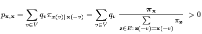
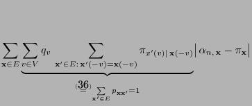
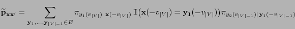
Let the transition matrix

be given
as
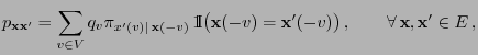 |
(36) |
where the conditional probabilities

are defined in

. Then

is
irreducible and aperiodic and the pair

is
reversible.
- Proof
-
The assertion can be proved similarly to the proof of
Theorem 3.10.
- In order to see that
is aperiodic it
suffices to notice
- that for all

- and hence all diagonal elements
 of
are
positive.
of
are
positive.
- The following considerations show that
is irreducible.
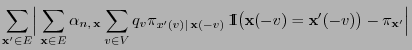
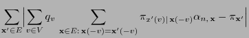
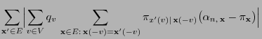
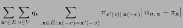
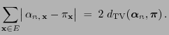
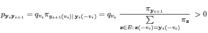
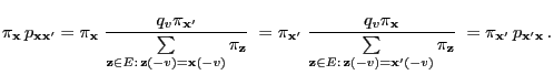
- It is left to show that the detailed balance equation
(2.85) holds, i.e.
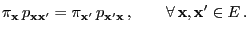 |
(38) |
Let
 be a Markov chain with state space
 and the transition matrix
given by (36). As a consequence of
Theorem 3.11 we get that in this case
and the transition matrix
given by (36). As a consequence of
Theorem 3.11 we get that in this case
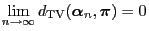 |
(39) |
for any initial concentration
 where
where
 denotes the distribution of
 . Furthermore, the Gibbs
sampler shows the following monotonic behavior.
. Furthermore, the Gibbs
sampler shows the following monotonic behavior.
- Proof
-
- Remarks
-
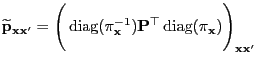
Theorem 3.13
The matrix

has the following
representation
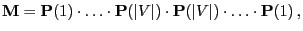 |
(45) |
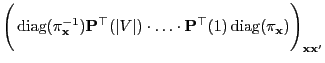
i.e., the multiplicative reversible version
of the
,,forward-scan matrix''
coincides with the
,,forward-backward scan matrix''.
- Proof
-
- Remarks
-
- If Gibbs samplers are used in practice it is always assumed
- The family
 of subsets of
  is called
a system of neighborhoods if for arbitrary
is called
a system of neighborhoods if for arbitrary 
- (a)
-
 ,
,
- (b)
-
 implies
 .
.
- For the hard-core model from Section 3.3.1,
 is the set of those vertices
  that are
directly connected to
that are
directly connected to  by an edge.
Next: Metropolis-Hastings Algorithm
Up: Simulation Methods Based on
Previous: Example: Hard-Core Model
Contents
Ursa Pantle
2006-07-20